Format Cell In Excel | Free Excel Tutorial

 Format Cells

In this chapter, we will discuss format cells, where we cover the following.

• Decimal Places
• Fractions
• Currency vs Accounting
• Text to Numbers
• Numbers to Text
• Custom Number Format
• Format Painter
• Cell Styles
• Wrap Text
• Merge Cells
• Strikethrough
• Superscript and Subscript
• Check Mark  

Let's start with the format of the cells, In Microsoft excel when we want to format cells, we change the view or appearance of any given number without changing the number itself. For example, we can set a number format  to 0.8, $0.80, 80%, or another formatting like alignment, font, border, etc

1. All a value "0.8"  into cell B2.

Microsoft Excel uses the General format by default like no specific number format for numbers. Use the 'Format Cells' dialog box to apply a number format.

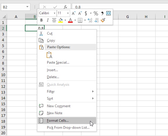
2. Select cell B2 and Right-click, and then click Format Cells or press CTRL + 1

 3.For example, select Currency.

Note: Excel will provide you a live preview of how the number will be formatted.

4. click ok and you will see the number is the format is changed to currency, with the number of the same steps can be changed into percentage number, etc.

We only changed the view of the number of cell B2 Cells. Frequently used formatting commands are available on the Home tab.

5. If you want to change the appearance of the number to percentage go to the Home tab, in the Number group, click the percentage symbol.

6. If you want to adjust the alignment of a number, Go to the Home tab, in the Alignment group, center the number, right the number, left the number.

7. By using the Font group in the Home tab, you can add outside borders and change the font color to any color.

Hopefully, this article will help you to enhance your knowledge of Mircosoft Excel. If you have any issues please let us know in the comment section or simply email me naeem.ahmed3034@gmail.com 

Excel Worksheet -Part 2 | Basic Excel | Mr. Excel

Excel Worksheet - Part 2

In this part of the Excel worksheet, we will discuss more parts, Zoom, Split, Freeze Pan. These all topics are related to Microsoft Excel worksheets or Excel spreadsheets. If you haven't read the first part of this topic, follow this link to get access to the first part.

https://mrexceluk.blogspot.com/2021/04/excel-worksheet.html

So let start the second part of the Excel Worksheet.

Zoom In Excel Worksheet.

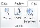
To zoom the document you can use the (- and +) icon in the status bar. You can also use the buttons in the view tab where you can adjust the zoom to a specific percentage.

You can follow these steps to adjust a specific Zoom percentage.

1- Go to the view tab and press the zoom icon, to set at 100% press the 100% button.

You can also perform zoom to selection with a button.

2- Select the percentage of zoom, or you can set it by custom percentage. 

How to Split the Excel worksheet.

You can split your Excel worksheet into panes like upper and lower.  To split your worksheet follow these steps.

1. Select the cell in Column A from where you want to split the screen.

2. Go to the View tab and select split in the window group.

3. You can check the worksheet is split into two panes upper and lower panes.

4. You can remove the split by double-clicking on the split bar.

5. You can split the horizontally by selecting the first cell of any column.

How to Freeze the Panes in Excel?

Freezing the rows or columns can be useful when you are working with a large table of data. Freezing the panes will allow you to see the rows or columns when you are scrolling the data in the worksheet area.

Freeze Top Row

If you want to freeze the top row of your worksheet, follow these steps.

1. Go to the View tab and click Freeze Panes in the Window group.

2. Click on Freeze top row.

3. Now you can check, you can scroll down in the worksheet, but your first row will remain on top and Excel will automatically add a horizontal line which will show that your top row is frozen now.

Unfreeze Panes

To unfreeze the frozen panes, follow these steps.

1. If you want to unfreeze the panes, go to the View tab and click Freeze Panes in the Window group.

2. Click on Unfreeze Panes and your panes will be unfrozen.

With the same action, you can freeze your first column and any column, any row, any cell by selecting that column, row, cell. You can get a magic freeze button on the top of the Quick Access toolbar by customizing it.

In the next part of this topic, we will explore more about Group worksheets, consolidate, Get Sheet name, spell check, view multiple sheets.

Excel Worksheet Part 1 

Excel Worksheet or Spreadsheet | Mr. Excel | Part-1

Excel Worksheet or Spreadsheet

what is excel worksheet or spreadsheet?

Also, Read Part-2 of this post.

Excel worksheet or spreadsheet is a collection of cells that are organized in rows and columns and where your data is displayed and stored. These worksheets or spreadsheets are a part of a workbook. A workbook can be based on many worksheets or spreadsheets. By default, a workbook contains 3 excel worksheets or spreadsheets in it I.e. "Sheet 1, Sheet2, Sheet 3", you can change the name of these sheets as per your choice. 

You can check the below screenshot as a display of an Excel worksheet or spreadsheet. Bullet numbers will elaborate on each and every part of a worksheet or spreadsheet.

• Cells are organized in columns and rows in the Excel worksheet. It's displayed as a rectangle grid in Excel worksheet.
• Rows are called vertical lines, each row has a label with numeric figures like 1-2-3-4, a worksheet contains a total of 1,048,576 rows or vertical lines.
• Columns are called horizontal lines, each column has a label with letters or alphabetic like A-B-C, there ere are 26 alphabet letters, the column labels start with A till Z for the first 26 columns, then labels  moves onto realignment like  AA, AB, AZ, BA, BB till ZZ, a worksheet contains 16384 columns or horizontal lines.
• Scroll Options are the symbols at the left and left bottom corners to scroll the sheet area in the Excel worksheet.

Cells & Columns in Excel

The cell in the Excel worksheet is also called the active cell. You can enter function or any new into the active cell from keyboard editing activity. The active cell can be identified in the Excel worksheet or spreadsheet by following points

When you click on a cell a black border (MS Excel 2010) or dark green border (MS Excel 365) will appear around it.

Column and row also highlighted with dark yellow colour (MS Excel 2010) or grey colour in (MS Excel 365).

In the top right corner of an active excel worksheet, the name box will appear as below. For example, you have clicked on a 3rd cell of "D" column it will be displayed "D3" in name box

Selecting A Worksheet in Excel

In a workbook only one worksheet will be visible which will be the active worksheet in Excel, From the bottom of the workbook you can select a different worksheet by clicking on it. You can use shortcut keys to select or change the active Excel worksheet, which are Ctrl + Page Up and Ctrl + Page Down 

Rename a worksheet in Excel.

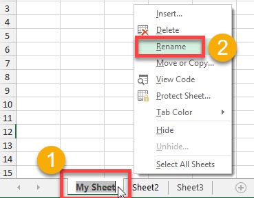
• Press mouse right-click on the sheet name (which sheet is to be renamed) in right bottom of sheets tab.
• Select rename option from the menu and edit it with new name with your keyboard editing.
• You can also rename the active worksheet in Excel by double clink on the sheet name which you want to rename.

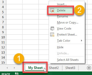
Delete a worksheet in Excel

• Press mouse right-click on the sheet (which sheet is to be deleted) in right bottom of sheets tab.
• Select delete option from the menu and delete the sheet from workbook
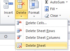
• You can also delete a worksheet by clicking on delete and then delete sheet from cells section in home tab.

Insert a worksheet.

• Right click on any active worksheet in Excel.
• Press right-click on mouse and then insert from the menu.
• You can also insert a worksheet by pressing the small plus (+) icon on the right side of all existing sheets.
• You can also insert a worksheet  by clicking on insert and then inset sheet from cells section in home tab.

 

Moving the Worksheet in Excel.

You can move the sheets into the any order which you like as per below screen short and bullet number process.

• Press Left-click(mouse or cursor) on the sheet which you want to move.
• Hold your cursor button down and drag the sheet which you want to move to the desired location where you want to move. 
• An icon of small worksheet will be  displayed while you are moving the sheet on new location.

Move Or Copy A Worksheet in Excel

You can use Move or Copy command from your mouse by press right-click on an active worksheet.

Hopefully this article will help you to enhance your basic excel skills, If you have required any assistance we are a click away, simply email me "naeem.ahmed3034@gmail.com"

Conclusion; 

Here we discussed worksheet, where we can make change several changes in it like rename, move, copy delete. Etc

Also, Read this : Create a new workbook in Excel.

Create a new workbook in excel - Mr. Excel

Create a new workbook in excel

What is workbook in excel?

Workbook in Excel, contains one or more worksheets or spreadsheets in a single file.  In short words your excel file is your workbook. A workbook have, rows, columns, status bar, cells, and many more in it as below.

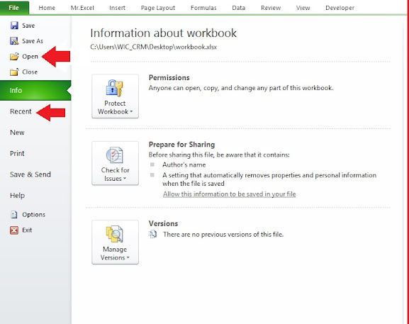
Open a Workbook.

If you want to open a workbook which is already saved in your PC, follow below steps.

1. Click on File tab (left top) and then click Open.

2. If you want to open your recent files on which you were working on past then click on file tab and then click recent files and choose the required file.

Create a New Workbook

If you want to create a new workbook, follow below steps.

1. Click on File tab (left top), click New.

2. Click Blank workbook if you want to create a blank workbook, you can create from templates, or you can download templates from office.com.

Themes

If you want to change the interface look of your workbook with one click, you can use the themes option in Excel workbook. Every theme contains 12 colors, 2 fonts(body and Headings), smart art and effects for shapes.

1. To change the theme click layout tab on ribbon, and then check themes group, by default workbook use standard office theme.

2. In the Home tab, you can see the font group, contains 2 fonts Cambria and Calibri, also you can see the theme colors of this theme.

You can customize the themes colors, fonts, or you can create a new theme as you required. You can use these themes in Microsoft Word or Microsoft PowerPoint.

Hopefully this article will enhance your basic excel skills. Feel free to contact in case of any help you need. We are just a click away, Please email me with your query regarding "workbook in excel",  naeem.ahmed3034@gmail.com    

Also, Read this : https://mrexceluk.blogspot.com/2021/04/checkbox-in-excel.html

Checkbox in excel - Free Online Excel Training with Mr. Excel

Check box in Excel

what is a checkbox in Excel?

Checkbox in Excel is tool that can be used to select or deselect an option in workbook. You can use a checkbox in Excel to create dashboards, checklists, and dynamic charts.

How to inset a checkbox in Excel?

Insert checkbox in Excel is a very easy and simple process. To insert a checkbox in excel worksheet, please follow these steps. 

1. Open the Developer tab, in the Controls group and click Insert.

2. Choose Check Box Form Controls section.

3. Draw checkbox on worksheet. You can delete or rename the checkbox by clicking on text.

How to link checkbox in Excel?

To link a checkbox, follow these steps.

1. Press Right click on checkbox and then click format control.

2. In control tab, make sure by default your checkbox is marked uncheck and then give reference to a cell where you want to link the checkbox because it will show the status as True and false.

3. Test the Checkbox, when you un check the box it will display "False" and if you check the box "True" will display a below. Our checkbox is working fine.

Create a Checklist

To create a checklist, follow these steps and watch video tutorial till end.

• Draw a checkbox in any cell.
• Click on the lower right corner of first cell and drag it down to cell where your products are. (For Example D2:D12 , where D2 is first and D12 is last), you can mannually set and align as describe in video tutorial.
• Right click on first checkbox and then click Format Control.
• Give reference cell link to  checkbox.
• Repeat same process (format control & reference cell link)  for all checkboxes.
• insert ROWS formula to count total products.
• Use COUNTIF formula to count the number of items packed.
• IF formula will be used to evaluate if you're good to go.
• Click all check boxes, and it will show you that you are good to go.
• Download sample file from below Link

Download Sample File

Also Read This : Status bar in excel

Status bar in Excel - Free Online Excel Training with MR.Excel

 

What is Status bar in Excel?

Status Bar in Excel

The Status Bar in Excel is the area which is at the very bottom in Excel which have special keys that are engaged can be seen or different information about the current mode. We can also select zoom in and out and different worksheet views on the worksheet from the status bar.

Status Bar

we will see number wise details in status bar as below.

1. In this tab we can see current mode and special keys information that are engaged. Here we are mentioning some extra features in bullet points

• More common modes include in number 1:
  • Ready mode is general status of Excel by default.
  • Enter mode is Currently entering content into a cell.
  • Edit mode is Currently editing a cell.
  • Extend Selection mode will see after pressing F8
  • Add to Selection mode will see after pressing SHIFT+F8.
• Some special keys like Caps Lock, Num Lock and Scroll Lock might be added.

2. Macro Recorder status tells us macro currently recording. We can start recording a macro by clicking this icon status and when we're done, we can stop recording by pressing again the icon status.

3. To open the customize status menu Right click anywhere in the status bar. We can select which items we want to show by checking them, and also we can hide the items which we do not want to show in the status bar.  Current statuses will also display on the right-hand side of the menu.

4.The Status Bar can be set to show summary of numerical values which we have selected in our workbook. 

5. Here you can select from three different worksheet views

• Normal view
• Page Layout view
• Page Break preview

6. Zoom Scroll Bar will allow us on the current working sheet, adjust the level of magnification.

7. Current Zoom Level will display the level of magnification on the worksheet on the current basis and when we will click it, it will open the Zoom menu to select the preset magnification options

Also Read : How to customize the ribbon?

Customize the ribbon in Excel - Free Online Training with Mr. Excel

How to customize ribbon in Excel?

Customize the ribbon

You can change the order of the default tabs, add custom tabs, rename tabs Customize the ribbon list,

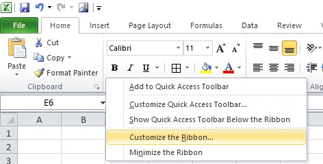
To customize the ribbon you have to right-click anywhere on the tabs' menu, Here's how you do that.

• Right Click anywhere on empty space in the ribbon 

Follow the steps below to customize the ribbon.

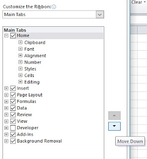
Change the order of default or custom tabs 

You can change the order of your existing tabs like Home, Insert, Draw, Design, and other tabs instead of File Only. Just select the tab which you want to move up or down and press up or down arrow keys as below.

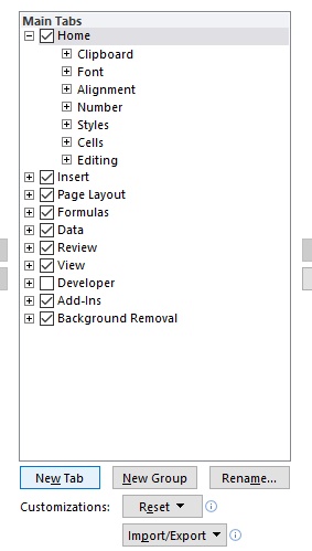
Add a custom tab or custom group: -Excel online

To add a custom tab or custom group, only commands will be added on custom tabs. In the window, under the Customize the Ribbon list, you will click on New Tab or New group and then press ok to save and see your changes

Rename a default or custom tab or custom group - Excel online

To rename a default or a custom tab or custom group in the Customize the ribbon window under the Customize the ribbon list, click the tab that you want to rename.

Now click Rename, and then type a new name that you want to appear on the ribbon. Press ok to save and see changes.

Hide a default or custom tab/custom group  -   Excel online

To hide both custom and default tabs please see below, you can only remove custom tabs. You cannot hide the File tab.

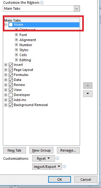
Simply clear the checkbox next to the default tab or custom tab that you want to hide. Click ok to see and save your changes.

Remove a custom tab/custom group

to hide both custom and default tabs, but you can only remove custom tabs.

Click the tab that you want to remove custom tabs, In in the Customize the ribbon window under the Customize the Ribbon list, and click remove. Click Ok to see and save your changes.

Hopefully, this article will help you to customize ribbon in Excel, please share your views or suggestions in the comment section. Your valued feedback is very important.

Developer tools in excel -Online Training with Mr. Excel

How to enable developer tools tab in excel?

How to enable developer tools tab in excel?

In this article we will discuss How to enable developer tools in Excel?

Excel developer tab is a built-in tab which is disabled by default, this tab provides the features which are necessary to us in  Visual Basic for Applications (VBA) and macro operations. To make it visible in the options section in the toolbar at the top of the Excel window.

Summary

• In Microsoft Excel, Developer tab is a key feature which is hidden by default.
• To create VBA applications, import and export XML data, create macros, design forms, etc.
• To appear on the toolbar of the Excel window, It must be enabled from the Options section by customize the ribbon

Importance of Developer Tab

Microsoft Excel is the best and one of the important application of Microsoft Office applications which are used by finance professionals and institutes. To create data reports, analyzing large data, making dashboards, etc. It's an easy application for bankers, data analysts, and institutes to make decisions quickly and easily.

Aforementioned professionals can check performance of companies, expected projections, and investment scenarios. After enabling Developer tab is in Excel, users can get more advanced functions like designing, creating macros, writing code, forms, importing and exporting XML file formats.

If you want to turn on the export and import XML files,  create a macro,  or insert controls you will be turned on developer tools first. To turn on the aforementioned tab, Please follow the steps.

1. First right-click on the ribbon, click Customize the ribbon. 

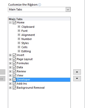
2. Below  Customize the Ribbon, see on the right side of the dialog box, select Main tabs (if necessary).

3. Mark check in the Developer check box.

3. Press ok to see and save changes 

4: After save changes you can check in developer options advance features are visible as below screenshot.

Hopefully this article will help you to  enable excel developer options, if you need any assistant regarding this article, or you are unable to open developer tab in Excel, you are just a click away me. Please email me naeem.ahmed3034@gmail.com